Geometric meaning of some inequalities with two variables

41

GEOMETRICAL MEANING OF SOME INEQUALITIES WITH TWO VARIABLES

A. Y. MARGULIS, B. A. RADUNSKY

When studying a mathematics course, a student often comes to solve inequalities and systems of inequalities with one unknown. At the same time, a geometric illustration of the solution (in combination with the method of integrals) helps them find the correct solutions in the shortest way.

Consider, for example, the inequality
$$\log_2 (x^2 - 4x + 3) \leq 3.$$
Its solution coincides with the solution to a system of two inequalities with one unknown
$$\begin{cases} x^2 - 4x + 3 > 0 \\ x^2 - 4x + 3 \leq 8 \end{cases}$$
(necessary for the existence of a logarithm),
(obtained by potentiating a given inequality).

The set of values ​​of $x$ satisfying the first inequality is a set of two integrals
$$x < 1 \text{ и } x > 3,$$
and the second - a segment
$$1 \leq x \leq 5$$
(this follows from the properties of the square triterm).

Having marked these intervals (Fig. 1) on the number axis, we see that the set of values ​​$x$ satisfying the system of inequalities fills two semi-closed integrals, $-1 \leq x < 1$ and $3 < x \leq 5$ (on figure they are given in the paragraph).

For greater clarity, on figure itself it is noted which of the ends of the integrals belong to the solution domain and which do not.

The geometric illustration turned out to be very useful here. Its role increases even more when solving inequalities and systems of inequalities with two unknowns.

42

Let us consider inequalities with two unknowns of the form

$$y - f(x) > 0.$$

(1)

Let’s construct a graph of the function $y = f(x)$ and take an arbitrary point $A'_1$ with the abscissa $x = x_0$ (Fig. 2). If, with the same $x = x_0$, its ordinate $y_1$ is greater than the ordinate $y_0$ corresponding to the point $A$ of the curve $y = f(x)$, then the point $A'_1$ lies above the curve. Point $A'_1$ lies under curve $y = f(x)$ if its ordinate $y_2$ is less than ordinate $y_0$. Therefore, the coordinates of all points lying below the curve $y = f(x)$ satisfy the inequality $y < f(x)$, and the coordinates of all points lying above the curve $y = f(x)$ satisfy the inequality $y > f(x)$.

Thus, the graph of the function $y = f(x)$ divides the coordinate plane into two parts, in one of which the inequality $y - f(x) > 0$ is satisfied, and in the other $y - f(x) < 0$.

Let us introduce the following definition. The power set of a plane is called convex if it, together with any two powers $A$ and $B$, contains all the powers of the segment $AB$.

Consider, for example, the interior of any triangle, circle, square. It can be shown that these sets are convex.

It is obvious that those parts into which the curve $y = f(x)$ divides the plane can be either convex or non-convex (see Fig. 2).

Let us now illustrate with a number of examples how using geometric concepts one can solve inequalities and systems of inequalities with two unknowns.

Consider the linear function $f(x) = ax + b$ (2).

The graph of the linear function $y = ax + b$ is a straight line (Fig. 3). This straight line divides the plane into two half-planes: upper and lower. In the first of them the inequality $y - (ax + b) > 0$ is satisfied, and in the second $y - (ax + b) < 0$. Note that both of these half-planes are convex sets.

43

Example 1. Find on the geometric coordinate plane the locations of points whose coordinates satisfy a system of two linear inequalities (solve graphical given systems of inequalities):

$$\begin{cases} y > -\frac{1}{2}x + 2, \\ y < -\frac{1}{2}x + 1; \end{cases}$$

$$\begin{cases} y > -\frac{1}{2}x + 1; \\ y < -\frac{1}{2}x + 2, \end{cases}$$

$$\begin{cases} y \geq \frac{1}{3}x + 1, \\ y \leq 2x - 2. \end{cases}$$

Solution. figure 4 shows graphical solutions to these inequalities. If the solution to each of the inequalities is colored yellow or gray, then the solution of the system is the part of the plane colored with both colors. From figure 4 it is clear that system a) has no solutions (Fig. 4,a); the solution of system b) is the half-plane lying above the line $y = -\frac{1}{2}x + 2$ (Fig. 4,b); the solution to system b) is an infinite strip between lines $y = -\frac{1}{2}x + 1$ and $y = -\frac{1}{2}x + 2$ (Fig. 4,c); and the solution to system d) is the part of the plane lying inside the double-shaded angle, including its sides (Fig. 4,d).

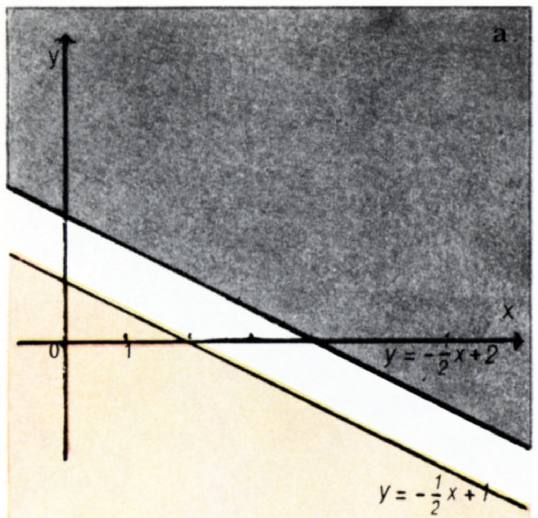
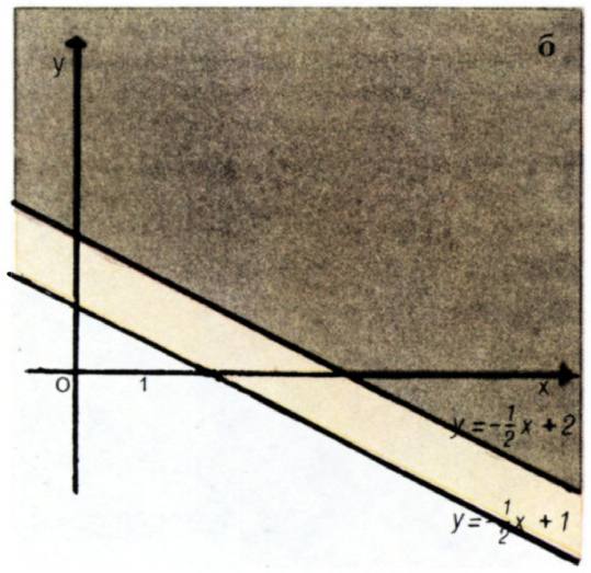
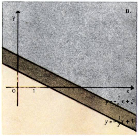
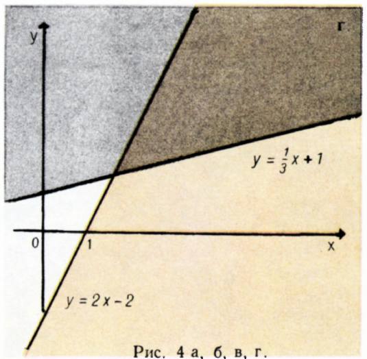
Fig. 4 a, b, c, d.

44

---

running_head:
folio:

Note that in all cases, the solution domains of a system of linear inequalities are convex sets. This is no coincidence. We have already noted that any straight line divides the plane into two convex sets, and the intersection (common part) of any number of convex sets is always a convex set.

Example 2. Solve graphically a system of three linear inequalities

$$\begin{cases} y < \frac{1}{3}x + 2, \\ y > -\frac{1}{2}x + 3, \\ y > 2x - 4. \end{cases}$$

Solution. This problem can be solved in the same way as the previous one. But due to the large number of restrictions, it is more convenient to paint not those areas where one or another inequality holds, but, on the contrary, those areas where there cannot be solutions. In this case, there is no need for different colors: after all, where at least one of the inequalities of the system is not satisfied, there cannot be solutions to the entire system. See figure 5 for a graphical solution to this example. The set of solutions is the set of interior points of triangle ABC. For clarity, the triangle is painted green.

To a system of linear property inequalities and some irrational and transcendental inequalities.

Example 3. Solve graphically the inequality $\sqrt{y-(x+1)}<1$.

Solution. The given inequality is equivalent to the following system of inequalities:

$$\begin{cases} y-(x+1) \geq 0 \\ y-(x+1) < 1 \end{cases}$$ or \begin{cases} y-(x+1) \geq 0, \\ y-(x+2) < 0.

The graphical solution of this example is shown on figure 6. Just as in example 3, the set of points satisfying this system is painted green. Primaya

45

$y = x + 1$, which belongs to the solution area, is drawn as a solid line, and the straight line $y = x + 2$, which does not belong to the solution area, is drawn as a dotted line.

Example 4. Solve graphical inequalities $\log_{y-1}(x-2) < 1$.

Solved and e. The range of permissible values ​​(APV) of unknowns is obviously determined by a system of inequalities

$$x > 2, y > 1, y \neq 2.$$

In accordance with this system, let us first eliminate the set that cannot have a solution. To do this, on figure 7 we paint half-plane $x < 2$, half-plane $y < 1$ with gray paint, and draw a straight line $y = 2$ with a dotted line.

Let’s now consider two cases:

a) $1 < y < 2$. Potentiating the original inequality, we obtain $x - 2 > y - 1$ or $y < x - 1$.

b) For $y > 2$ we get $x - 2 < y - 1, y > x - 1$.

The solutions corresponding to these cases are shown in green on figure7.

Solve examples 5 and 6 on your own.

Example 5. Solve graphical inequalities $\log_{y-1}(y - x + 2) > 0$ (see Fig. 8).

Example 6. Solve graphical inequalities $\log_x \log_y y > 0$ (see Fig. 9).

Let us now consider the square three-fold

$$f(x) = ax^2 + bx + c.$$

As is known, the graph of the function $y = ax^2 + bx + c$ is a parabola with an axis of symmetry parallel to the ordinat axis and with a vertex at point $B\left(-\frac{b}{2a}, -\frac{D}{4a}\right)$, where $D = b^2 - 4ac$.

The graph of one of the quadratic trinomials (at $a > 0$) is shown schematically in figure 10. This graph divides the plane into two parts, in one of which the inequality $y - (ax^2 + bx + c) > 0$ holds, and in the other $y - (ax^2 + bx + c) < 0$. Reader without difficulty

46

Let him notice that only one of these parts is a convex set.

Example 7. Solve graphical inequalities $\log_y(5x-x^2-6)>1$.

Solution i.e. The range of admissible values ​​is obviously determined by the inequalities

$$\begin{cases} 5x-x^2-6>0, \\ y>0, \\ y\neq 1. \end{cases}$$

The first of these inequalities is equivalent to the inequality $x^2-5x+6<0$. Its solutions fill the interval $2<x<3$.

On figure 11, those parts of the plane where $x<2$ and $x>3$ are shaded with gray, resulting in $y<0$, and the points lying on the dotted line $y=1$ are also excluded.

Let’s consider two cases: $y>1$ and $0<y<1$.

a) $y>1$. Potentiating the original expression, we obtain the inequality $5x-x^2-6>y$, or $y-(-x^2+5x-6)<0$. The last inequality is satisfied by the coordinates of all points located under the parabola $y=-x^2+5x-6$, but none of them corresponds to the conditions $y>1$. Thus, for $y>1$ there are no solutions.

b) $0<y<1$. Similarly, we obtain the inequality $5x-x^2-6<y$, i.e. $y-(-x^2+5x-6)>0$.

Obviously, the solution is the area above the parabola $y=-x^2+5x-6$ shaded green at figure 11.

Solve examples 8 and 9 yourself.

Example 8. Solve graphical inequalities $\sqrt{y}<x-1$ (see Fig. 12).

Example 9. Solve graphical inequalities (see Fig. 13)

$$\left(\frac{1}{3}\right)^{x-1} > \left(\frac{1}{3}\right)^{\sqrt{y-x+3}}$$

Example 10. Solve graphical inequalities

$$\sqrt{1-(x-3)^2-(y-2)^2} < \sqrt{1-(x-4)^2-(y-2)^2}$$

Solution i.e. In this case, the ODZ is determined by the inequalities

47

$$\begin{align*} 1 - (x - 3)^2 - (y - 2)^2 &\geq 0, \\ 1 - (x - 4)^2 - (y - 2)^2 &\geq 0. \end{align*}$$

or

$$\begin{align*} (x - 3)^2 + (y - 2)^2 &\leq 1, \\ (x - 4)^2 + (y - 2)^2 &\leq 1. \end{align*}$$

The equation $(x - 3)^2 + (y - 2)^2 = 1$ is the equation of a circle of unit radius centered at the point $O_1(3;2)$. The inequality $(x - 3)^2 + (y - 2)^2 \leq 1$ is satisfied by all points distant from the point $O_1$ by no more than one, that is, all points of the indicated circle, including its boundary. The set of points whose coordinates satisfy the second unknown is defined similarly and is the common part of two circles (Fig. 14). It remains to find the set of points for which the given inequality holds. After estimated transformations, we obtain inequalities that in this ODZ are equivalent to the original one:

$$\begin{align*} 1 - (x - 3)^2 - (y - 2)^2 &< \\ < 1 - (x - 4)^2 - (y - 2)^2, \\ (x - 4)^2 - (x - 3)^2 &< 0, \\ x &>\frac{7}{2}. \end{align*}$$

Thus, the solution is the area painted on figure 14 with it (the part of the ODZ lying to the right of the straight line $x = \frac{7}{2}$).

Finally, consider the following example.

Example 11. Among the points whose coordinates satisfy the condition $x + 2y \leq 3$, $2x - y \leq 1$, $x \geq 0$ and $y \geq 0$, find a point for which the expression $x^2 + y^2$ will be the most accurate.