Attention: there is a parameter in the equation!

20

In terms of parameters, the distance of all possible cases is of particular importance. At the same time, it is difficult to predict in advance which cases will emerge during the decision process. This, on the one hand, complicates the solution, but, on the other hand, makes the work more interesting, giving it a research character.

A little theory

The general form of an equation with one parameter is:
$$F(x,a) = 0.$$ (3)

For different $a$, equation (3) can have different sets of roots, and our task is to study all cases, find out what will happen for any value of the parameter. When solving an equation with a parameter, you usually come to consider many different options. Timely detection of at least some of the impossible options is of great importance, as it frees us from unnecessary work. Therefore, when solving equation (3), it is advisable to understand by OD the range of permissible values ​​of the unknown and the parameter, that is, the set of all pairs of numbers $(x,a)$ for which the function of two variables $F(x,a)$ is defined (makes sense). Hence the natural geometric illustration of the ODZ in the form of a certain region of the $xOa$ plane.

For example, the ODZ equation
$$\sqrt{x} + \sqrt{a} = \sqrt{1-(x+a)}$$ (4)
determined by the system of inequalities
$$x \geq 0, a \geq 0, x+a \leq 1.$$

This system is satisfied by the coordinates of all points of the triangle (including its boundaries), surrounded by figure 1 in blue and blue colors *). From these considerations, by the way, it immediately follows that for $a<0$ equation (4) has no solution.

Let’s solve equation (4). After squaring both of its parts (which in this case is an equivalent transformation due to the non-negativity of both sides of equation (4)), we obtain the equation
$$2\sqrt{ax} = 1 - 2(x+a).$$ (5)

We already said above that discarding at least part of the impossible options frees us from unnecessary work. We note that the left side of equation (5) is non-negative for all admissible $a,x$, which means that where the right side of this equation is negative, it is useless to look for a solution. It is clear that solutions should be sought in that part of the ODZ where they can be, by making an appropriate narrowing of the ODZ for this purpose:
$$1 - 2(x+a) \geq 0, \text{ откуда } x+a \leq \frac{1}{2}.$$

At figure 1, the part of the ODZ where there cannot be a solution is painted with the removed color.

By squaring both sides of equation (5) **) and bringing similar terms, we obtain the equation
$$x^2 + (a-1)x + a^2 - a + \frac{1}{4} = 0,$$

*) For more information about the geometric solution to a system of inequalities with two unknowns, see «Kvant» No. 4 for 1970.
**) In the new ODZ both sides of equation (5) are non-negative. In this case, squaring will not lead to the appearance of constructed roots.

21

where
$$x_{1,2} = \frac{1-a \pm \sqrt{2a-3a^2}}{2}.$$

Both found roots for all admissible values ​​of the parameter $a$, (that is, for all $a$ satisfying the inequalities $0 \leq a \leq \frac{1}{2}$ - see figure 1) are real numbers. Indeed, the discriminant $D = 2a-3a^2 \geq 0$ for $0 \leq a \leq \frac{2}{3}$; that means, even more so $D \geq 0$ with $0 \leq a \leq \frac{1}{2}$.

Now we need to find out whether the found values ​​satisfy the conditions $x \geq 0$, $x+a \leq \frac{1}{2}$.

Let us first check that condition $x+a \leq \frac{1}{2}$ is met. We have
$$x_1+a = \frac{1-a-\sqrt{2a-3a^2}}{2} + a = \frac{1+a-\sqrt{2a-3a^2}}{2}.$$
Solving inequality
$$\frac{1+a-\sqrt{2a-3a^2}}{2} \leq \frac{1}{2},$$
we get $0 \leq a \leq \frac{1}{2}$. This means $x_1+a \leq \frac{1}{2}$ for all admissible values ​​of the parameter $a$.

Next,
$$x_2+a = \frac{1-a+\sqrt{2a-3a^2}}{2} + a = \frac{1+a+\sqrt{2a-3a^2}}{2}.$$
Inequality
$$\frac{1+a+\sqrt{2a-3a^2}}{2} \leq \frac{1}{2}$$

is executed only at $a = 0$. But for $a = 0$ we have $D = 0$ and $x_1=x_2 = \frac{1}{2}$.

The proof of the non-negativity of both found roots is left to the reader.

Answer: if $0 \leq a \leq \frac{1}{2}$, then $x = \frac{1-a-\sqrt{2a-3a^2}}{2}$;

if $a < 0$ or $a > \frac{1}{2}$, then there are no solutions.

Note that when solving the equation considered, drying of the ODZ turns out to be useful. The question naturally arises: when should such clarifications be made?

If we carry out a transformation that results in an equation equivalent to the previous one, then in the case of ODZ there is, of course, no need. Otherwise it is useful. This situation arises, for example, when squaring (or to any even power) both parts of an equation, which is what we encountered in the example considered.

Some examples
Example 1*). Solve the equation
$$\frac{\sqrt{a+x}}{a} + \frac{\sqrt{a+x}}{x} = \sqrt{x}.$$
Solution. The ODZ is determined by the equations $x > 0$, $a+x \geq 0$, $a \neq 0$ (from here, by the way, it immediately follows that at $a = 0$ the equation has no solution). Let’s transform the equation to the form
$$(a+x)^{3/2} = ax^{3/2}.$$
Let’s dry the ODZ: from the non-negativity part of the last equation and the equations $x > 0$, $a \neq 0$ it follows that $a > 0$.

Next we get: $a+x = a^{2/3}x$, from where $x (a^{2/3}-1) = a$.
With $a = 1$ there are very/no solutions. If $a \neq 1$, then
$$x = \frac{a}{a^{2/3}-1}.$$
Let’s find out whether, with everyone’s consideration,
*) No. 206 from the “Collection of problems in elementary mathematics.” Authors: N. P. Antonov, M. Ya. Vygodsky, V. V. Nikitin, A. I. Sankin. In the given problem the example is solved/herno.

22

---

running_head:
folio:

Given the values ​​of the parameter $a$ ($a > 0, a \neq 1$), condition $x > 0$ is satisfied (from which it obviously follows that the second condition $a + x \geq 0$ is satisfied).

The inequality $\frac{a}{a^{2/3} - 1} > 0$ holds only for $a > 1$ (taking into account that $a > 0$). Thus, not for all admissible values ​​of $a$ the found root turns out to be suitable.

Answer: if $a > 1$, then $x = \frac{a}{a^{2/3} - 1}$; if $a \leq 1$, then there is no solution.

Example 2: Solve the equation
$$\log_9 x + \log_9 \frac{2 - x}{2} = \log_9 \log_9 p.$$

Solution. The ODZ is determined by the inequalities $0 < x < 2$, $p > 1$ (at figure 2 this area is colored crimson). Solving the equation, we consistently obtain
$$\frac{x(2 - x)}{2} = \log_9 p,$$
$$x^2 - 2x + 2\log_9 p = 0,$$
$$x_{1,2} = 1 \pm \sqrt{1 - 2\log_9 p}.$$

Condition $1 - 2\log_9 p \geq 0$ is satisfied for $p \leq 3$, which, taking into account the ODZ, gives $1 < p \leq 3$. With such $p$ the roots will be real numbers. At $p > 1$ the inequality $\log_9 p > 0$ is satisfied, and then $1 - 2\log_9 p < 1$. It follows that for $1 < p \leq 3$ the inequality $0 < x_{1,2} < 2$ holds.

Answer: if $1 < p \leq 3$, then $x_{1,2} = 1 \pm \sqrt{1 - 2\log_9 p}$; for the remaining $p$ there are no solutions.

Comment. From equation (6) we obtain $p = 9^{\frac{x(2 - x)}{2}}$. The graph of this function, plotted on figure 2, clearly shows that the condition $0 < x < 2$ is satisfied at $1 < p \leq 3$.

Example 3: Solve the equation
$$\frac{a + \sin x}{a \cos x + 1} = \frac{a + \cos x}{a \sin x + 1}.$$

Solution. Let us first consider the case $a = 0$. The given equation takes the form $\sin x = \cos x$, hence $x = \frac{\pi}{4} + \pi n$ ($n = 0, \pm 1, \ldots$).

Let now $a \neq 0$. Then the ODZ is determined by the equations
$$\cos x \neq -\frac{1}{a}; \sin x \neq -\frac{1}{a}.$$

Let us transform the given equation to the form $(\sin x - \cos x)[a^2 + a(\sin x + \cos x) + 1] = 0$. The last property equation is to the following set of equations:
$$a^2 + a(\sin x + \cos x) + 1 = 0,$$
$$\sin x - \cos x = 0.$$

Solving the first equation of the set (7), we obtain:
$$a\sqrt{2}\sin(x + \frac{\pi}{4}) = -a^2 - 1$$
and onwards
$$\sin\left(x + \frac{\pi}{4}\right) = -\frac{a^2 + 1}{a\sqrt{2}}.$$

The last equation has no solution, since $\left| -\frac{a^2 + 1}{a\sqrt{2}} \right| > 1$ for any $a \neq 0$. Indeed, suppose that $\frac{a^2 + 1}{|a|\sqrt{2}} \leq 1$; transforming this inequality, we get
$$a^2 + 1 \leq |a|\sqrt{2}, (a^2 + 1)^2 \leq 2a^2,$$
$$a^4 + 1 \leq 0.$$

The last inequality is incorrect.

23

The solutions to the second population equation (7) are the values ​​$x = \frac{\pi}{4} + \pi k$ ($k = 0, \pm 1, \ldots$). It remains to check whether, for all values ​​of $a \neq 0$, the found values ​​of $x$ are admissible.

If $k = 2n$, then $\sin x = \cos x = \frac{\sqrt{2}}{2}$ and the condition $\frac{\sqrt{2}}{2} \neq -\frac{1}{a}$ must be satisfied, that is, $a \neq -\sqrt{2}$.

If $k = 2n + 1$, then $\sin x = \cos x = -\frac{\sqrt{2}}{2}$.

From the condition $-\frac{\sqrt{2}}{2} \neq -\frac{1}{a}$ we obtain: $a \neq \sqrt{2}$.

Combining all the results, write

Answer: if $a \neq \pm \sqrt{2}$, then $x = \frac{\pi}{4} + \pi k$;

if $a = \sqrt{2}$, then $x = \frac{\pi}{4} + 2\pi n$;

if $a = -\sqrt{2}$, then $x = \frac{\pi}{4} + \pi (2n + 1)$ ($k,n = 0, \pm 1, \pm 2; \ldots$).

Example 4. Solve equation $\log^2_{\sqrt{2}} \cos x - 2a \log_{\sqrt{2}} \cos x = a^2 - 8$.

(8)

Solution. Putting $y = \log_{\sqrt{2}} \cos x$, we transform the given equation into a quadratic equation $y^2 - 2ay - (a^2 - 8) = 0$,

whence $y_{1,2} = a \pm \sqrt{2(a^2 - 4)}$.

Now we need to solve a set of logarithmic equations

$$\log_{\sqrt{2}} \cos x = a + \sqrt{2(a^2 - 4)}. \tag{9}$$

$$\log_{\sqrt{2}} \cos x = a - \sqrt{2(a^2 - 4)}. \tag{10}$$

We note that for $a^2 - 4 < 0$ the right-hand sides of equations (9) and (10) do not make sense. This means that, for $-2 < a < 2$, both equations have no solutions. Consider the case $a^2 - 4 \geq 0$, which is possible with $a \geq 2$ or with $a \leq -2$.

Let’s start with $a \geq 2$. Since $\cos x \leq 1$ and $\sqrt{2} > 1$, then $\log_{\sqrt{2}} \cos x \leq 0$.

This means that equations (9) and (10) will have solutions only for such values ​​of the parameter $a$ for which the right-hand sides of the equation are non-positive. It is easy to see that for $a \geq 2$ the right-hand side of equation (9) is positive, therefore, equation (9) has no solutions.

Let us find out at what values ​​of the parameter $a$ the right-hand side of equation (10) will be non-positive. Solving the inequality $a - \sqrt{2(a^2 - 4)} \leq 0$ (taking into account the condition $a \geq 2$), we obtain $a \geq \sqrt{8}$. Thus, if $2 \leq a < \sqrt{8}$, then equation (10) has no solutions (and since equation (9) also has no solutions, we conclude from this that equation (8) in this case also has no solutions).

If $a \geq \sqrt{8}$, then from equation (10) we obtain

$$x = \pm \arccos(\sqrt{2})^{a - \sqrt{2(a^2 - 8)}} + 2\pi n. \tag{11}$$

Let us now consider the case $a \leq -2$. For these parameter values, the right side of equation (10) is different, that is, this equation has solutions (they are already written above by formula (11)). Let us find out at what values ​​of the parameter $a$ the right-hand side of equation (9) will be non-positive. Solving the inequality $a + \sqrt{2(a^2 - 4)} \leq 0$ (taking into account the condition $a \leq -2$), we obtain $a \geq -\sqrt{8}$. Thus, if $a < -\sqrt{8}$, then equation (9) has no solutions, if $-\sqrt{8} \leq a \leq -2$, then equation (9) has solutions, namely:

$$x = \pm \arccos(\sqrt{2})^{a + \sqrt{2(a^2 - 8)}} + 2\pi n.$$

Combining all the results obtained, we write down

Answer: if $-2 < a < \sqrt{8}$, then there are no solutions;

if $a \geq \sqrt{8}$ or $a < -\sqrt{8}$ then

$$x = \pm \arccos(\sqrt{2})^{a - \sqrt{2(a^2 - 8)}} + 2\pi n;$$

if $-\sqrt{8} \leq a \leq -2$, then

24

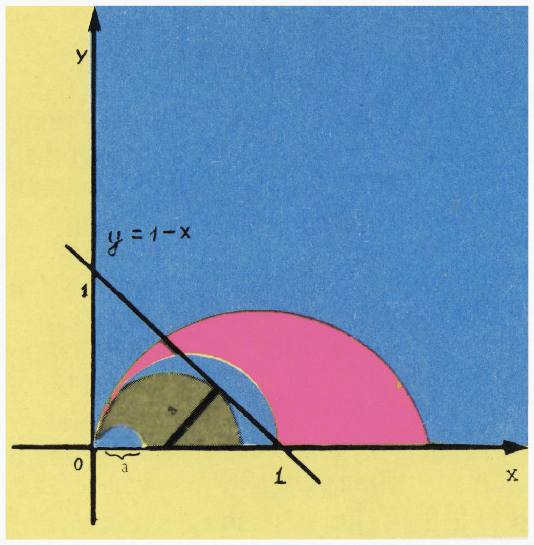
Fig. 3.

$$x = \pm \arccos(\sqrt{2})^{a \pm \sqrt{2}a^2 - 8} + 2\pi n.$$

Geometry helps algebra

When solving an equation with a parameter, various geometric considerations may be useful for scales. Consider, for example, the equation

$$\sqrt{x(2a-x)} = 1 - x \text{ при } a > 0.$$

Which solution of the equation can be interpreted as the abscissa of the point of intersection of the straight line $y = 1 - x$ with the semicircle

$$y = \sqrt{x(2a-x)}, \text{ или}$$
$$(x - a)^2 + y^2 = a^2; \text{ у} \geq 0$$

radius $a$, centered at point $(a, 0)$ (Fig. 3). The position of the semicircle and its radius change as the parameter $a$ changes. On figure 3 it is clearly visible that for some values of $a$ the semicircle does not intersect the line $y = 1 - x$ (semicircles lying under the line), for other values $a$ the semicircle intersects the line at two points (semicircles lying in the middle head zone), for third values $a$ the semicircle intersects the line at one point (semicircles lying in the red zone or above), and for some values of $a$ the semicircle touches the line (semicircle separating the head and brown zones).

Let us consider the case when the semicircle touches the line $y = 1 - x$. From geometric considerations we conclude that the distance of the center of this semicircle from the point of intersection of the straight line $y = 1 - x$ with the abscissa axis is equal to $a\sqrt{2}$. Hence $a + a\sqrt{2} = 1$, that is, the case of tangency occurs at $a = \sqrt{2} - 1$. This means that at $a < \sqrt{2} - 1$ the equation has no solution (blue zone), but at $a = \sqrt{2} - 1$ it has a unique solution, which is found from geometric considerations: $x = a + \frac{a\sqrt{2}}{2}$ (see Fig. 3), from which we obtain $x = \frac{\sqrt{2}}{2}$.

The semicircle passing at figure 3 through the point $(1, 0)$ corresponds to the value of the parameter $a = \frac{1}{2}$. This means that for $\sqrt{2} - 1 < a \leqslant \frac{1}{2}$ the equation has two solutions:

$$x_1 = \frac{a + 1 - \sqrt{a^2 + 2a - 1}}{2},$$
$$x_2 = \frac{a + 1 + \sqrt{a^2 + 2a - 1}}{2}$$

(the roots are found using an algebraic solution to the given equation). Finally, if $a \geqslant \frac{1}{2}$, then the equation has a unique solution $x = x_1$ (since $x_1 < x_2$).

25

Answer: if $a < \sqrt{2} - 1$, then there are no solutions;
if $a = \sqrt{2} - 1$, then $x = \frac{\sqrt{2}}{2}$;
if $\sqrt{2} - 1 < a \leq \frac{1}{2}$,
then $x_{1,2} = \frac{a+1 \pm \sqrt{a^2+2a-1}}{2}$.

If
$a > \frac{1}{2}$, then $x = \frac{a+1 - \sqrt{a^2+2a-1}}{2}$.

Try to solve the proposed algebraic equation yourself with the corresponding research, and you will see that geometric reasoning in this case is both clearer and more beautiful.

TASKS

We looked at a number of examples of solving an equation with one parameter. Some of you liked them more, others less, but one thing is certain: if you carefully examined these examples with a pencil in your hands (as the editorial collection of our magazine advised in No. 1), then you have already received the definition of creep. Want to make sure of this? Solve the following equation yourself with parameter $a$:

1. $a^2 - \frac{a^2-1}{2x-x^2} = \frac{x+2}{x-2}$.
2. $\sqrt{x+a} = a - \sqrt{x}$.
3. $\sqrt{x-2a} - \sqrt{x-a} = 2$.
4. $x + \sqrt{x^2-x} = a$.
5. $\sin(a+x) + \sin x = \cos \frac{a}{2}$.
6. $\sin^2 x + 4 \sin x + a = 0$.
7. $\sin x + 2 \cos ax = 3$.
8. $\log_{\sqrt{x}} a \log_{a^2} \frac{a^2-4}{2a-x} = 1$.
9. $\frac{\log_x(2a-x)}{\log_x 2} + \frac{\log_a \sqrt{x}}{\log_a 2} = \frac{1}{\log_{a^2}-1}$.
10. $\log_{\frac{1}{2}}(2 \sin x) + a \log_{\frac{1}{2}} \sin x + 3 = 0$.

4 Quantum No. 9